KonigCell Tutorials#
Rasterizations using KonigCell can be done in a couple of ways:
Dynamic trajectories / static particles.
2D pixels / 3D voxels.
Splitting a raster’s values across cells (
konigcell.mode) - this is more subtle, see below.
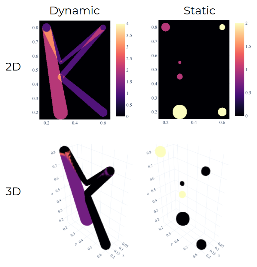
The code for generating these frames is given in the Basic Tutorials section.
Rasterization Modes#
Given a particle moving between positions [P1, P2, P3, …], we will rasterize given values [V1, V2, V3, …] onto a 2D / 3D grid. The values can be any particle property - velocity, time taken to move between two locations, etc.
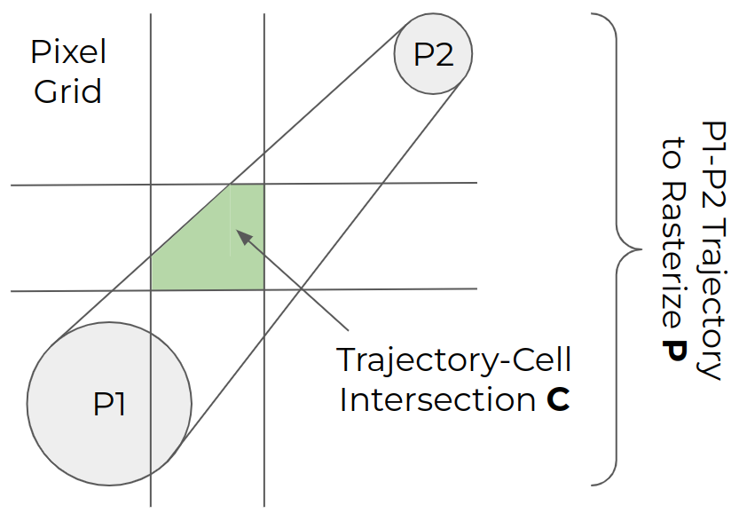
For a dynamic particle moving between positions P1 and P2, we will rasterize value V1 onto the grid of cells. But what value should each cell contain?
Let the area shaded by the particle moving between P1 and P2 be P; the area intersected by
P and a given grid cell is C. The rasterization mode determines what value the
intersected grid cell should have:
kc.ONE- add the value V1; e.g. velocity.kc.PARTICLE- add the value V1 * P.kc.INTERSECTION- add the value V1 * C.kc.RATIO- add the value V1 * C / P; e.g. time spent should be split across each intersection.
Here is an accelerating particle moving in an inward spiral, rasterizing its velocity using different modes:
